Cloud Masking: Why a Binary Choice Breaks a Continuous Problem
2025-08-09 · 9 min read · Cloud Masking · Cloud Shadows · Sentinel-2 · Sen2Cor

TL;DR: Clouds, haze, and shadows are continuous, not binary. Prefer probabilistic scores plus geometry and time-aware fusion, and only hard-mask when you truly must.
Most teams start with a cloud bitmask because it feels clean: Either a pixel is usable or it is not. That is also where the trouble starts. The atmosphere rarely cooperates with clean categories, and the cost of forcing a threshold shows up immediately as either holes in your map or subtle contamination that quietly biases your numbers.
If you do monitoring, change detection, or any kind of time series, this trade-off is unavoidable. Your only real choice is whether you handle it explicitly (probabilities, weighting, multi-date logic) or let a binary mask handle it implicitly (and unpredictably) via gaps and flicker.
Why cloud masking is a spectrum problem
Real scenes do not split neatly into “cloud” and “clear.” You will meet thin cirrus, low stratus and fog, broken cumulus fields, stratocumulus decks, bright snow and ice, salt flats, bright sand, sunglint on water, smoke and dust, and adjacency effects near cloud edges.
Many modern detectors output a cloud probability score per pixel. The moment you pick a threshold, you inherit a coverage-versus-contamination trade-off: Raise the threshold and you keep more pixels (plus more haze and cloud edges). Lower it and you reduce contamination (plus you punch more holes).
The same is true for cloud shadows. A shadow is low signal, not zero. Over dark water and evergreen forest, shadows blend into real surface variability unless you bring in geometry and context.
Cloud types that punish hard thresholds
Deep convective cumulus and cumulonimbus. These are the “easy” clouds visually, but they create hard geometry problems. Bright tops plus large displaced shadows mean that a small error in estimated cloud height can move a shadow projection by many pixels, and high clouds introduce parallax that shifts apparent cloud position across view angles.
Stratocumulus decks. Textured sheets with semi-transparent breaks generate edge ambiguity. Conservative dilation removes fringes but also deletes valid pixels, while permissive thresholds keep coverage but leak bright edges that bias reflectance and indices.
Thin cirrus and subvisible cirrus. High-altitude ice clouds transmit light and reduce contrast while leaving apparent structure below. Sentinel-2 includes a dedicated cirrus band (Band 10, about 1.375 μm) specifically to support cirrus detection.Sentinel-2 User Handbook (Copernicus): Band 10 at 1.375 μm enables cirrus detection In the Sen2Cor Level-2A algorithm, cirrus detection relies on per-pixel Band 10 reflectance thresholds under daytime viewing conditions.Sentinel-2 Level-2A Algorithm ATBD: cirrus detection uses Band 10 reflectance thresholds Even with this help, thin cirrus can slip through simple visible tests and still depress vegetation signals.
Low stratus and fog. These can be spectrally similar to bright surfaces, especially over snow, salt pans, and beaches. Thermal bands (common on Landsat) help separate temperature-driven ambiguity, but Sentinel-2 MSI does not include thermal bands, so you lean harder on visible and shortwave infrared (SWIR) cues plus texture and terrain context.USGS FAQ: Sentinel-2 MSI excludes Landsat thermal bands
Smoke and dust. Aerosols are not clouds, but they can look cloud-like in single-date optical data. Optically thin smoke can be usable for some tasks if you treat it as lower-confidence rather than “bad,” while dust over bright land is one of the fastest ways to make fixed thresholds lie.
Cloud-shadow detection works better as geometry first
Shadow logic is usually more reliable when you treat it as a projection problem, not a spectral one. You project likely shadow regions along the sun vector using solar azimuth and zenith, sensor geometry, and an estimate of cloud-top height. In mountainous terrain you often need a DEM (digital elevation model).
Most shadow failures are boring and repeatable: Height underestimation projects shadows too short and misses the real dark area, height overestimation projects shadows beyond the dark patch and steals valid pixels, and terrain plus parallax shifts everything just enough to create persistent “shadow noise” in a time series. Spectral checks can still help, but they work best as a confirmation step after geometry, not as the primary detector.
Look-alikes: bright land, glint, snow, and haze
Hard masks struggle most where the surface naturally resembles cloud or shadow in parts of the spectrum. Bright deserts, beaches, gypsum, and salt pans can trip “white equals cloud” logic unless you use SWIR cues and texture. Urban roofs and concrete can be spectrally flat and bright enough to look cloud-like in visible bands. Snow and ice are high-albedo surfaces with their own edge cases, especially in complex terrain where topographic shadows and mixed pixels flicker across dates. Water adds sunglint and whitecaps, where reflectance depends heavily on geometry and wind conditions.
If you only take one lesson from these cases, make it this: A “cloud mask” is often solving a broader “non-ideal pixel” problem, and many of those pixels are still useful if your pipeline can express uncertainty instead of dropping them.
What common cloud masking workflows actually output
Popular workflows vary, but many follow the same pattern: Compute intermediate tests and scores, then publish a single binary decision.
Fmask is a rule-based workflow that combines multiple spectral tests and object-based steps to label cloud, cloud shadow, and snow, including versions adapted for Sentinel-2 imagery.Zhu & Woodcock (Remote Sensing of Environment, 2015): Fmask improvements and Sentinel-2 adaptation Sen2Cor produces a Scene Classification Layer (SCL) and quality indicators that include cloud and snow probabilities as part of Level-2A processing.Sen2Cor Quick Guide: outputs include SCL and quality indicators including cloud and snow probabilities s2cloudless is widely used to generate a per-pixel cloud probability layer for Sentinel-2, and it still requires thresholds and post-processing choices once you turn probabilities into a mask.sentinel2-cloud-detector (s2cloudless) GitHub repository
So the “binary mask problem” is not that detectors are naive. It is that many pipelines collapse uncertainty into a single bit too early, then act surprised when the world refuses to stay binary.
Working with probabilities instead of hard masks
A practical way out is to delay the hard decision. Keep the per-pixel cloud (and shadow) probability as a first-class signal and use it as a weight. Pixels with medium probability are not automatically thrown away; they are treated as less trustworthy in downstream steps like compositing, smoothing, change detection, or model inference.
This also makes thresholds less dramatic. You can still publish a binary mask for compatibility, but your internal logic can use soft rules like “prefer low-probability pixels when available” rather than “delete everything above X.” That is how you reduce flicker and stop edge pixels from whiplashing your time series.
Temporal fusion without losing the nominal date
When you need a clean map “for today,” the temptation is to crank thresholds until clouds are gone. That often backfires by creating holes that are worse than light haze.
A more reliable pattern is to keep a nominal date but allow limited, local support from nearby dates. If a pixel is questionable today, compare it with a recent clear observation and either downweight today’s value or substitute a nearby-date value under a tight time window, depending on the application.
This is not a free lunch. You have to handle co-registration, changing illumination, and genuine surface change. But it is usually easier than pretending a single date can always be perfectly cloud-free.
How ClearSKY approaches uncertainty in cloud masking
ClearSKY’s data fusion is built to rely less on binary cloud masking, because binary masking throws away exactly the pixels you often want to keep: Thin cloud, cloud-edge pixels, haze, and shadows. In practice, we use multiple models depending on region, season, and task, and we try to keep uncertainty in the pipeline rather than collapsing it into a single “good or bad” switch.
The goal is not to “ignore clouds.” The goal is to use less-than-perfect imagery when it is still informative, and to let fusion across time and modalities carry the load instead of aggressive hard thresholds. That is how you keep coverage high without pretending that every kept pixel is equally trustworthy.
Quick view: cloud type vs masking pitfalls
| Cloud or condition | What breaks masks | Typical false positives | Useful cues to fix |
|---|---|---|---|
| Deep cumulus and cumulonimbus | Long displaced shadows, parallax, bright tops | Dark water or forest labeled as shadow | Shadow geometry with height brackets, SWIR absorption tests, DEM-aware projection |
| Stratocumulus decks | Edge pixels, subpixel gaps, adjacency brightening | Bright sand or urban roofs at edges | Moderate dilation, texture and gradient checks, adaptive thresholds |
| Thin cirrus | Partial transmission with low contrast | Haze or smoke over water | 1.38 μm cirrus band on Sentinel-2, multi-date consistency, spectral slope tests |
| Low stratus and fog | Spectral confusion with bright surfaces | Snow, salt flats, beaches | Thermal on Landsat, SWIR and coastal aerosol on Sentinel-2, terrain context |
| Smoke and dust | Variable spectra and texture | Thin cloud classification over land and water | Blue-to-SWIR ratios, temporal persistence, plume morphology |
| Snow and ice | High albedo with complex terrain shadows | Cloud over mountains, cloud edges over snow | NDSI (normalized difference snow index), terrain shadow modeling, BRDF (bidirectional reflectance distribution function) awareness |
| Water with sunglint | Specular streaks and whitecaps | Cloud over oceans and lakes | Glint modeling, NIR (near-infrared) and SWIR checks, wind and geometry awareness |
FAQ
›What is cloud masking in satellite imagery?
Cloud masking is the process of identifying pixels likely affected by clouds, cloud edges, or cloud shadows so they can be excluded or treated differently. Many systems publish the result as a binary bitmask, but most modern methods start by estimating a probability or confidence. The important detail is when your pipeline turns that confidence into a hard keep-or-drop decision.
›Why do binary masks cause gaps or contamination?
Because the underlying signal is not binary. A strict threshold removes thin cloud and haze but also deletes usable pixels, creating holes and time-series flicker. A permissive threshold keeps coverage high but lets in veiling haze or cloud edges that bias reflectance and derived indices.
›How should I choose a cloud probability threshold?
Choose it based on the cost of errors in your application, not on what looks nicest in a viewer. If false change alarms are expensive, you usually want stricter handling of uncertain pixels. If missing data is the bigger problem, you will get better results by keeping medium-confidence pixels but downweighting them and leaning on temporal support.
›Are cloud shadows just another class to mask?
Not really. Shadows behave like a geometry problem first, because their location depends on sun angles, cloud height, and terrain. Spectral checks help, but without geometry you will keep confusing dark surfaces with shadows or missing real shadows that shift with parallax and relief.
›Is it ever OK to keep pixels under thin clouds or haze?
Yes, if your downstream method can represent uncertainty. Thin cloud, haze, and even some shadows can still preserve enough structure for tasks like relative monitoring or feature detection, especially when combined with nearby-date context. The mistake is treating every kept pixel as equally clean, which is exactly what a binary mask encourages.